
Scale-Up Domains and the Fabric Boundary: Designing Past One Rack
Overview
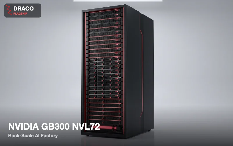
The single most consequential architectural parameter in a rack-scale AI system is the size of its scale-up domain — the set of GPUs connected by NVLink, inside which bandwidth is measured in terabytes per second, versus everything beyond it, where bandwidth drops by roughly an order of magnitude. GB300 NVL72 gives 72 GPUs in that domain; Vera Rubin NVL144 gives 144; Kyber is expected to give 576. Getting your model’s parallelism to align with that boundary is worth more than a generational jump in accelerator speed, and misaligning it wastes a substantial fraction of a very expensive machine.
Key takeaways
- Scale-up and scale-out differ by roughly an order of magnitude in bandwidth, and more in latency behaviour.
- Tensor and expert parallelism belong inside the domain; data and pipeline parallelism can cross it.
- Crossing the boundary with the wrong dimension is the most common cause of disappointing multi-rack throughput.
- Domain size is growing fast — 72 to 144 to a reported 576 across three generations.
- Measure achieved bandwidth per parallel dimension, not aggregate cluster FLOPS.
Two networks, not one
Inside a rack-scale system, NVLink and its switches form a fabric where any GPU can reach any other at very high bandwidth with low, predictable latency. It behaves close to a shared memory system for collective operations. Outside the rack, InfiniBand or Ethernet connects racks into a cluster, and while modern scale-out fabrics are fast, they are not in the same class — and their latency characteristics under congestion differ fundamentally.
The distinction is not merely quantitative. Collective operations that complete predictably inside the scale-up domain become sensitive to congestion, routing and tail latency when they cross the boundary. A model that runs at high utilisation within one rack can drop sharply when the same parallelism spans two, and the cause is usually not average bandwidth but variance.
Mapping parallelism to the boundary
| Parallelism | Communication pattern | Frequency | Where it belongs |
|---|---|---|---|
| Tensor parallel | All-reduce within each layer | Very high | Inside the scale-up domain |
| Expert parallel (MoE) | All-to-all token routing | Very high | Inside the scale-up domain |
| Sequence or context parallel | Exchange across sequence chunks | High | Inside, preferably |
| Pipeline parallel | Point-to-point activations between stages | Moderate | Can cross the boundary |
| Data parallel | Gradient all-reduce per step | Once per step | Crosses the boundary well |
This table is effectively the design rule. Tensor and expert parallelism communicate within every layer and must stay on the fast fabric. Data parallelism communicates once per optimisation step and tolerates a slower network, particularly with gradient compression and overlap. Pipeline parallelism sits between: point-to-point transfers are less demanding than all-reduce, but pipeline bubbles hurt utilisation independently.
Why the boundary decides your configuration
Given a model, the required tensor-parallel degree follows from its layer widths and memory footprint. If that degree fits inside the scale-up domain, you configure data parallelism across racks and the system behaves well. If it does not, you either accept tensor parallelism crossing the boundary — which is where throughput collapses — or introduce pipeline parallelism to reduce the tensor degree, which brings bubbles instead.
This is why domain growth matters more than its FLOPS implications suggest. A model needing tensor-parallel degree 16 is comfortable on a 72-GPU domain. One needing degree 128 is not, and on a 144-GPU domain it becomes straightforward. The generational comparison is developed in Vera Rubin NVL144 and the following step in Rubin Ultra and Kyber NVL576.
Planning a multi-rack deployment
Four steps. Determine the minimum tensor-parallel degree your model requires from its architecture and memory footprint at the precision you will use. Confirm it fits inside one scale-up domain; if not, revisit precision, sharding strategy or model choice before revisiting hardware. Assign data parallelism across racks, sized so the gradient all-reduce can overlap with computation. And validate the scale-out fabric under real collective load rather than with a point-to-point bandwidth test, since problems appear at scale that no pairwise test reveals.
The topology rules for the scale-out layer have not changed and are covered in GPU cluster networking: rail-optimised connectivity, non-blocking within a scalable unit, and oversubscription only at aggregation where the traffic pattern justifies it.
Inference has the same boundary, different pressure
For serving rather than training, the same rule applies with a different emphasis. A model that fits within one node’s memory needs no cross-node communication at all, which is the cheapest and most reliable configuration. A model requiring tensor parallelism across GPUs should keep that within the scale-up domain, and a model too large for one domain forces a design decision that materially affects latency.
Disaggregated serving changes the calculus, because prefill and decode can be separated across different hardware with only KV cache transferred between them — a much lighter communication pattern than tensor-parallel all-reduce. That is one reason the architecture described in disaggregated inference has become standard for large-model serving: it converts a bandwidth problem into a scheduling problem.
What to measure
Aggregate cluster FLOPS tells you nothing useful about whether a configuration will work. Three measurements do. Achieved all-reduce bandwidth at your tensor-parallel degree, measured on the actual hardware and topology. Step time variance across ranks, which exposes whether a collective is crossing a boundary it should not. And scaling efficiency — throughput at N racks divided by N times single-rack throughput — which should stay high if the parallelism is mapped correctly and degrades sharply if it is not.
A scaling efficiency that falls off steeply between one and two racks is nearly always a boundary-crossing problem rather than a fabric problem, and the fix is usually reconfiguration rather than more hardware. The broader goodput framing is in training goodput at 10,000 GPUs.
Frequently asked questions
What is a scale-up domain?
The set of GPUs connected by NVLink and its switches within a rack-scale system, inside which any GPU reaches any other at very high bandwidth with predictable latency. Beyond it, InfiniBand or Ethernet connects racks at roughly an order of magnitude less bandwidth.
Which parallelism must stay inside the domain?
Tensor parallelism and expert parallelism, because both communicate within every layer — all-reduce and all-to-all respectively. Data parallelism communicates once per step and crosses the boundary well; pipeline parallelism sits between the two.
Why does throughput collapse when tensor parallelism crosses racks?
Because a per-layer all-reduce becomes sensitive to congestion, routing and tail latency on the scale-out fabric. The problem is often variance rather than average bandwidth, and it compounds across every layer of every step.
How do I know if my configuration is mapped correctly?
Measure scaling efficiency — throughput at N racks over N times single-rack throughput. A steep fall between one and two racks almost always indicates a parallel dimension crossing the boundary, which is fixed by reconfiguration rather than more hardware.
Does this apply to inference as well?
Yes, with different emphasis. Keeping a model within one node or one scale-up domain avoids cross-boundary communication entirely. Disaggregated serving helps by separating prefill and decode with only KV cache transferred, which is far lighter than tensor-parallel all-reduce.
Ready to deploy?
Talk to an RDP architect about power, cooling and lead time.